 计量经济学实验报告.docx
- 文档编号:7989799
- 上传时间:2023-05-12
- 格式:DOCX
- 页数:24
- 大小:68KB
计量经济学实验报告.docx
《计量经济学实验报告.docx》由会员分享,可在线阅读,更多相关《计量经济学实验报告.docx(24页珍藏版)》请在冰点文库上搜索。
计量经济学实验报告
计量经济学实验报告
专业国际经济与贸易班级一班姓名姜祥丽学号20114913
实验一
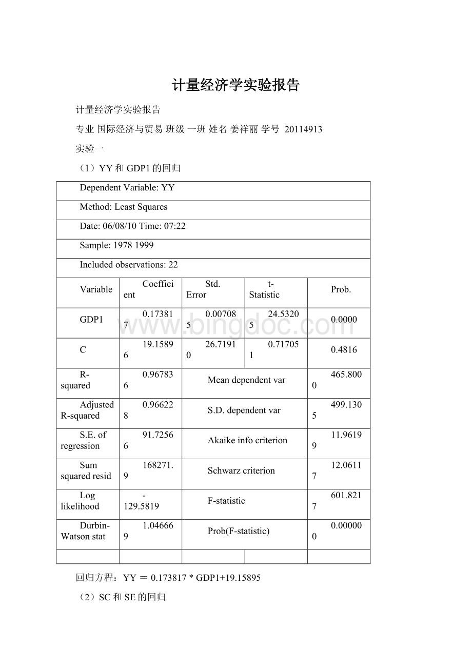
(1)YY和GDP1的回归
DependentVariable:
YY
Method:
LeastSquares
Date:
06/08/10Time:
07:
22
Sample:
19781999
Includedobservations:
22
Variable
Coefficient
Std.Error
t-Statistic
Prob.
GDP1
0.173817
0.007085
24.53205
0.0000
C
19.15896
26.71910
0.717051
0.4816
R-squared
0.967836
Meandependentvar
465.8000
AdjustedR-squared
0.966228
S.D.dependentvar
499.1305
S.E.ofregression
91.72566
Akaikeinfocriterion
11.96199
Sumsquaredresid
168271.9
Schwarzcriterion
12.06117
Loglikelihood
-129.5819
F-statistic
601.8217
Durbin-Watsonstat
1.046669
Prob(F-statistic)
0.000000
回归方程:
YY=0.173817*GDP1+19.15895
(2)SC和SE的回归
DependentVariable:
CS
Method:
LeastSquares
Date:
06/08/10Time:
07:
27
Sample:
19781999
Includedobservations:
22
Variable
Coefficient
Std.Error
t-Statistic
Prob.
SE
0.482249
0.016112
29.93042
0.0000
C
31.03074
9.401733
3.300534
0.0036
R-squared
0.978162
Meandependentvar
215.8573
AdjustedR-squared
0.977070
S.D.dependentvar
219.5927
S.E.ofregression
33.25218
Akaikeinfocriterion
9.932625
Sumsquaredresid
22114.15
Schwarzcriterion
10.03181
Loglikelihood
-107.2589
F-statistic
895.8303
Durbin-Watsonstat
1.274578
Prob(F-statistic)
0.000000
回归方程:
CS=31.03074+0.482249*SE
实验二
(一)REV=-5826.158+0.084781035*GDP
(2517.475)(0.003311)
(-2.314286)(25.60453)
R2=0.976176SE=7732.823
DependentVariable:
REV
Method:
LeastSquares
Date:
06/08/10Time:
08:
04
Sample:
19781995
Includedobservations:
18
Variable
Coefficient
Std.Error
t-Statistic
Prob.
GDP
0.084781
0.003311
25.60453
0.0000
C
-5826.158
2517.475
-2.314286
0.0343
R-squared
0.976176
Meandependentvar
38637.72
AdjustedR-squared
0.974687
S.D.dependentvar
48603.38
S.E.ofregression
7732.823
Akaikeinfocriterion
20.84877
Sumsquaredresid
9.57E+08
Schwarzcriterion
20.94771
Loglikelihood
-185.6390
F-statistic
655.5922
Durbin-Watsonstat
0.335513
Prob(F-statistic)
0.000000
经济意义检验:
财政收人REV对国内生产总值GDP的回归系数为0.084781,无论从参数的符合和大小来说都符合经济理论。
说明国内生产总值GDP增加1个单位,财政收人REV增加0.085个单位。
统计检验:
根据数据的统计方程,判定系数R2接近1,拟合优度较高;参数显著性t检验拒绝犯错的概率为0,即拒绝原假设,通过t检验,GDP对REV有显著性影响。
常数C的t检验的概率为0.034小于0.05,所以通过t检验。
(二)EXB=(-2457.310)+(0.719308)*REV
(680.5738)(0.011153)
(-3.610644)(64.49707)
R2=0.996168SE=2234.939
DependentVariable:
EXB
Method:
LeastSquares
Date:
06/08/10Time:
07:
44
Sample:
19781995
Includedobservations:
18
Variable
Coefficient
Std.Error
t-Statistic
Prob.
REV
0.719308
0.011153
64.49707
0.0000
C
-2457.310
680.5738
-3.610644
0.0023
R-squared
0.996168
Meandependentvar
25335.11
AdjustedR-squared
0.995929
S.D.dependentvar
35027.97
S.E.ofregression
2234.939
Akaikeinfocriterion
18.36626
Sumsquaredresid
79919268
Schwarzcriterion
18.46519
Loglikelihood
-163.2963
F-statistic
4159.872
Durbin-Watsonstat
2.181183
Prob(F-statistic)
0.000000
经济意义检验:
财政支出EXB对财政收入REV的回归系数为0.719308,无论从参数的符合和大小来说都符合经济理论。
说明财政收人REV增加1个单位,财政支出EXB平均增加0.72个单位。
统计检验:
根据数据的统计方程,判定系数R2接近1,拟合优度较高;参数显著性t检验拒绝犯错的概率为0,即拒绝原假设,通过t检验,REV对EXB有显著性影响。
常数C的t检验的概率为0.0023小于0.05,所以通过t检验。
(三)SLC=(-2411.361)+(0.431827)*GDP
(3076.237)(0.004046)
(-0.783857)(106.7267)
R2=0.998597SE=9449.149
DependentVariable:
SLC
Method:
LeastSquares
Date:
06/08/10Time:
08:
05
Sample:
19781995
Includedobservations:
18
Variable
Coefficient
Std.Error
t-Statistic
Prob.
GDP
0.431827
0.004046
106.7267
0.0000
C
-2411.361
3076.237
-0.783867
0.4446
R-squared
0.998597
Meandependentvar
224062.6
AdjustedR-squared
0.998510
S.D.dependentvar
244763.3
S.E.ofregression
9449.149
Akaikeinfocriterion
21.24968
Sumsquaredresid
1.43E+09
Schwarzcriterion
21.34861
Loglikelihood
-189.2471
F-statistic
11390.59
Durbin-Watsonstat
1.715091
Prob(F-statistic)
0.000000
经济意义检验:
社会消费品零售额SLC对国内生产总值GDP的回归系数为0.431827,无论从参数的符合和大小来说都符合经济理论。
说明国内生成总值GDP增加1个单位,社会消费品零售额SLC分别平均增加0.432个单位。
统计检验:
根据数据的统计方程,判定系数R2接近1,拟合优度较高;参数显著性t检验拒绝犯错的概率为0,即拒绝原假设,通过t检验,GDP对SLC有显著性影响。
常数C的t检验的概率为0.4446大于0.05,所以没有通过t检验。
实验三
(一)把ZJ作为应变量,GDP1和T作为两个解释变量进行二元线性回归分析。
1、分别做ZJ和GDP1、ZJ和T的散点图:
分析:
从散点图看,变量之间不一定呈现线性关系
2、多元线性回归
DependentVariable:
ZJ
Method:
LeastSquares
Date:
03/31/13Time:
18:
40
Sample:
19781999
Includedobservations:
22
Variable
Coefficient
Std.Error
t-Statistic
Prob.
T
-6.728731
1.235938
-5.444229
0.0000
GDP1
0.176471
0.004305
40.99647
0.0000
R-squared
0.995817
Meandependentvar
378.1314
AdjustedR-squared
0.995608
S.D.dependentvar
458.5207
S.E.ofregression
30.38617
Akaikeinfocriterion
9.752360
Sumsquaredresid
18466.38
Schwarzcriterion
9.851546
Loglikelihood
-105.2760
F-statistic
4761.733
Durbin-Watsonstat
0.848685
Prob(F-statistic)
0.000000
得到估计方程为:
ZJ=0.17647447*GDP1+6.7287292*T
分析:
估计方程的调整判定系数为0.995608接近于1,所以拟合优度较高;方程显著性F检验拒绝犯错的概率为0,说明拒绝原假设,即方程显著性F检验显著;参数显著性t检验拒绝犯错的概率都为0,即拒绝原假设,通过t检验。
(二)把SE作为应变量,GDP1和T作为两个解释变量进行二元线性回归分析。
1、分别做SE与GDP1、SE与T的散点图:
分析:
从散点图看,变量之间不一定呈现线性关系
2、多元线性回归
DependentVariable:
SE
Method:
LeastSquares
Date:
03/31/13Time:
18:
03
Sample:
19781999
Includedobservations:
22
Variable
Coefficient
Std.Error
t-Statistic
Prob.
GDP1
0.169558
0.002925
57.97489
0.0000
T
-4.712952
0.839743
-5.612372
0.0000
R-squared
0.997998
Meandependentvar
383.2595
AdjustedR-squared
0.997898
S.D.dependentvar
450.3519
S.E.ofregression
20.64551
Akaikeinfocriterion
8.979381
Sumsquaredresid
8524.746
Schwarzcriterion
9.078567
Loglikelihood
-96.77319
F-statistic
9972.446
Durbin-Watsonstat
0.566752
Prob(F-statistic)
0.000000
得到估计方程为:
SE=0.16955751*GDP1+4.7129508*T
分析:
估计方程的调整判定系数为0.997898接近于1,所以拟合优度较高;方程显著性F检验拒绝犯错的概率为0,说明拒绝原假设,即方程显著性F检验显著;参数显著性t检验拒绝犯错的概率都为0,即拒绝原假设,通过t检验。
实验四
要求一:
做ZJ对GDP1和T回归的残差趋势图和残差散点图。
结论:
从图上看ZJ对GDP1、T回归的残差存在异方差。
要求二:
做对ZJ和GDP1回归的Glejser检验。
(1)abs(e1)与GDP1做回归
DependentVariable:
ABS(E1)
Method:
LeastSquares
Date:
06/22/10Time:
08:
00
Sample:
19782000
Includedobservations:
23
Variable
Coefficient
Std.Error
t-Statistic
Prob.
GDP1
0.004387
0.001443
3.040305
0.0062
C
20.71896
6.063898
3.416773
0.0026
R-squared
0.305635
Meandependentvar
33.34424
AdjustedR-squared
0.272570
S.D.dependentvar
24.84736
S.E.ofregression
21.19219
Akaikeinfocriterion
9.028084
Sumsquaredresid
9431.287
Schwarzcriterion
9.126822
Loglikelihood
-101.8230
F-statistic
9.243454
Durbin-Watsonstat
1.148496
Prob(F-statistic)
0.006221
从F检验来看整个模型显著
(2)abs(e1)与GDP1^2做回归
DependentVariable:
ABS(E1)
Method:
LeastSquares
Date:
06/22/10Time:
08:
02
Sample:
19782000
Includedobservations:
23
Variable
Coefficient
Std.Error
t-Statistic
Prob.
GDP1^2
4.82E-07
1.64E-07
2.928548
0.0080
C
24.83660
5.329758
4.659985
0.0001
R-squared
0.289974
Meandependentvar
33.34424
AdjustedR-squared
0.256164
S.D.dependentvar
24.84736
S.E.ofregression
21.42984
Akaikeinfocriterion
9.050387
Sumsquaredresid
9643.999
Schwarzcriterion
9.149126
Loglikelihood
-102.0794
F-statistic
8.576393
Durbin-Watsonstat
1.132628
Prob(F-statistic)
0.008028
从F检验来看整个模型显著
(3)abs(e1)与SQR(GDP1)做回归
DependentVariable:
ABS(E1)
Method:
LeastSquares
Date:
06/22/10Time:
08:
03
Sample:
19782000
Includedobservations:
23
Variable
Coefficient
Std.Error
t-Statistic
Prob.
SQR(GDP1)
0.464073
0.158455
2.928736
0.0080
C
12.16515
8.500612
1.431091
0.1671
R-squared
0.290001
Meandependentvar
33.34424
AdjustedR-squared
0.256191
S.D.dependentvar
24.84736
S.E.ofregression
21.42944
Akaikeinfocriterion
9.050350
Sumsquaredresid
9643.639
Schwarzcriterion
9.149088
Loglikelihood
-102.0790
F-statistic
8.577497
Durbin-Watsonstat
1.118705
Prob(F-statistic)
0.008024
常数项不显著,去掉常数项再进行回归得结果为:
DependentVariable:
ABS(E1)
Method:
LeastSquares
Date:
06/22/10Time:
08:
08
Sample:
19782000
Includedobservations:
23
Variable
Coefficient
Std.Error
t-Statistic
Prob.
SQR(GDP1)
0.656981
0.085253
7.706276
0.0000
R-squared
0.220758
Meandependentvar
33.34424
AdjustedR-squared
0.220758
S.D.dependentvar
24.84736
S.E.ofregression
21.93392
Akaikeinfocriterion
9.056451
Sumsquaredresid
10584.13
Schwarzcriterion
9.105820
Loglikelihood
-103.1492
Durbin-Watsonstat
1.019181
(4)abs(e1)与1/GDP1做回归
DependentVariable:
ABS(E1)
Method:
LeastSquares
Date:
06/22/10Time:
08:
04
Sample:
19782000
Includedobservations:
23
Variable
Coefficient
Std.Error
t-Statistic
Prob.
1/GDP1
-3994.363
3218.612
-1.241020
0.2283
C
39.30882
7.021346
5.598474
0.0000
R-squared
0.068328
Meandependentvar
33.34424
AdjustedR-squared
0.023963
S.D.dependentvar
24.84736
S.E.ofregression
24.54784
Akaikeinfocriterion
9.322066
Sumsquaredresid
12654.53
Schwarzcriterion
9.420805
Loglikelihood
-105.2038
F-statistic
1.540131
Durbin-Watsonstat
0.869730
Prob(F-statistic)
0.228283
从F检验来看整个模型不显著
从四个回归的结果看,回归(4)不显著,
(1)
(2)(3)显著,比较
(1)
(2)与(3)不带常数项的回归,还是选择
(1),方程为:
ABS(resid)=0.004387GDP1+20.71896
所以异方差的形式为:
σi2=σ2(GDP1)2
要求三:
已知ZJ对GDP1回归异方差的形式为:
把
作为权数来进行加权最小二乘法。
得到回归结果为:
DependentVariable:
ZJ
Method:
LeastSquares
Date:
06/22/10Time:
08:
24
Sample:
19782000
Includedobservations:
23
Weightingseries:
1/(GDP1^(1/6))
Variable
Coefficient
Std.Error
t-Statistic
Prob.
GDP1
0.162521
0.002949
55.11028
0.0000
C
-31.09968
9.069704
-3.428963
0.0025
WeightedStatistics
R-squared
0.990759
Meandependentvar
339.9230
AdjustedR-squared
0.990319
S.D.dependentva


- 配套讲稿:
如PPT文件的首页显示word图标,表示该PPT已包含配套word讲稿。双击word图标可打开word文档。
- 特殊限制:
部分文档作品中含有的国旗、国徽等图片,仅作为作品整体效果示例展示,禁止商用。设计者仅对作品中独创性部分享有著作权。
- 关 键 词:
- 计量 经济学 实验 报告
 冰点文库所有资源均是用户自行上传分享,仅供网友学习交流,未经上传用户书面授权,请勿作他用。
 《d t n l》公开课教案优秀教学设计5.docx
-
《大禹治水》公开课教案优秀教学设计14.docx
-
《父与子》读后感10篇.docx
-
《红星美凯龙物业管理部安全操作手册》.docx
-
《白杨》公开课教案和教学反思.docx
-
《动物临床诊疗技术》课程标准.docx
-
《广州市建设工程监理合同》SF0206.docx
-
《安全系统工程第三版徐志胜版》课后答案.docx
-
《动画运动规律》课程教案模板.docx
-
《管理学原理》综合测验考试复习资料.docx
-
《计算机网络》实验指导书修改版.docx
-
《平行四边形的面积》教学设计8.docx
-
《生药学》课程指导书.docx
-
《闻一多先生的说和做》阅读练习含答案.docx
-
《易经系辞》通讲二十七.docx
-
《坐井观天》教学实录与评析教案文档资料.docx
-
《悲歌行》.docx
-
《窦娥冤》导学案.docx
-
《广州市商品房买卖合同预售示范文本》SF0102.docx
-
《计算机应用基础》练习题含答案.docx
-
《企业信息管理》形成性作业有答案版.docx
-
《食品安全法》试题答案.docx
-
《我的母亲》课后练习题答案.docx
-
《英雄》电影观后感.docx
-
0Hnsjy大学英语四级真题听力原文.docx
-
02冬期雨期施工措施.docx
-
3安徽理工大学人人大使团.docx
-
5 外币业务会计处理 练习.docx
-
07年下学期教师法制学习资料.docx
-
09货币政策.docx
-
10第九章 会议礼仪.docx
-
12温度与物态变化教学案讲解.docx
-
五年职业规划范文复习过程.docx
-
下半年人力资源管理师三级理论知识真题.docx
-
小班科学探索小水滴旅行记doc.docx
-
小学期中表彰大会校长讲话稿doc.docx
-
效用理论.docx
-
新教材人教版地理必修一第三章第二节海水的性质同步练习含答案.docx
-
徐汇区华泾镇地块项目策划书.docx
-
学校第28个爱国卫生月活动方案.docx
-
阳极氧化膜的电解着色.docx
-
一建工程经济计算公式汇总及计算题解析.docx
-
仪器仪表常用英语词汇.docx
-
英语浙江省丽水市英语中考真题.docx
-
有关竞争的事例.docx
-
云南茶叶产业发展的基本情况.docx
-
浙江专用高考英语大一轮新优化复习Unit3TheMillionPoundBankNote课件新人.docx
-
执业药师药事管理与法规检测试题1完整篇doc.docx
-
中国玉米产消量供需平衡情况玉米价格走势及市场演变进程分析.docx
-
中心学校与学校领导签订一岗双责责任书知识讲解.docx
-
注册共用设备工程师暖通专业知识点整理.docx
