 《计量经济学》实验报告.docx
- 文档编号:4618181
- 上传时间:2023-05-07
- 格式:DOCX
- 页数:18
- 大小:25.59KB
《计量经济学》实验报告.docx
《《计量经济学》实验报告.docx》由会员分享,可在线阅读,更多相关《《计量经济学》实验报告.docx(18页珍藏版)》请在冰点文库上搜索。
《计量经济学》实验报告
计量经济学
实
验
报
告
学号1111111111
姓名xxx
专业班级软件1101班
指导老师xx
日期20xx年xx月
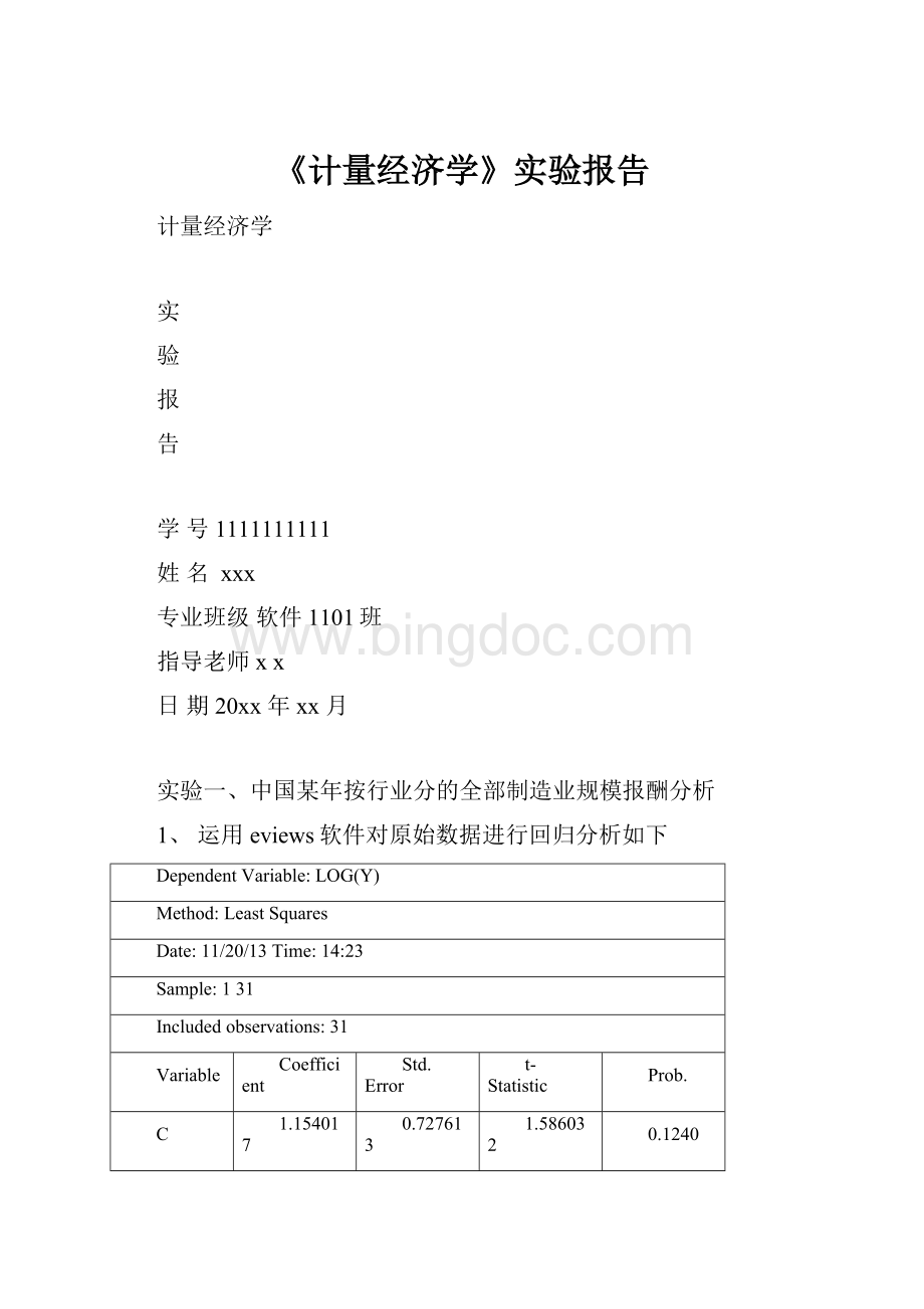
实验一、中国某年按行业分的全部制造业规模报酬分析
1、运用eviews软件对原始数据进行回归分析如下
DependentVariable:
LOG(Y)
Method:
LeastSquares
Date:
11/20/13Time:
14:
23
Sample:
131
Includedobservations:
31
Variable
Coefficient
Std.Error
t-Statistic
Prob.
C
1.154017
0.727613
1.586032
0.1240
LOG(K)
0.609232
0.176378
3.454120
0.0018
LOG(L)
0.360799
0.201592
1.789752
0.0843
R-squared
0.809924
Meandependentvar
7.494001
AdjustedR-squared
0.796347
S.D.dependentvar
0.942959
S.E.ofregression
0.425538
Akaikeinfocriterion
1.220842
Sumsquaredresid
5.070322
Schwarzcriterion
1.359615
Loglikelihood
-15.92306
F-statistic
59.65458
Durbin-Watsonstat
0.793198
Prob(F-statistic)
0.000000
2、参数检验模型估计
DependentVariable:
LOG(Y/L)
Method:
LeastSquares
Date:
11/20/13Time:
14:
30
Sample:
131
Includedobservations:
31
Variable
Coefficient
Std.Error
t-Statistic
Prob.
C
1.026065
0.596770
1.719365
0.0962
LOG(K/L)
0.608138
0.173590
3.503294
0.0015
R-squared
0.297363
Meandependentvar
3.100044
AdjustedR-squared
0.273134
S.D.dependentvar
0.491331
S.E.ofregression
0.418892
Akaikeinfocriterion
1.159931
Sumsquaredresid
5.088634
Schwarzcriterion
1.252447
Loglikelihood
-15.97894
F-statistic
12.27307
Durbin-Watsonstat
0.846451
Prob(F-statistic)
0.001511
实验二、某年中国部分城镇家庭平均可支配收入与消费性支出研究
1、利用eviews软件分析(图示法)
2、Eviews软件下载,OLS的估计结果如下
DependentVariable:
Y
Method:
LeastSquares
Date:
11/20/13Time:
14:
39
Sample:
120
Includedobservations:
20
Variable
Coefficient
Std.Error
t-Statistic
Prob.
C
272.3635
159.6773
1.705713
0.1053
X
0.755125
0.023316
32.38690
0.0000
R-squared
0.983129
Meandependentvar
5199.514
AdjustedR-squared
0.982192
S.D.dependentvar
1625.275
S.E.ofregression
216.8900
Akaikeinfocriterion
13.69130
Sumsquaredresid
846743.0
Schwarzcriterion
13.79087
Loglikelihood
-134.9130
F-statistic
1048.912
Durbin-Watsonstat
1.670234
Prob(F-statistic)
0.000000
3、异方差检验
a、首先进行GQ检验:
对X从大到小排列,却掉中间4个,对前后两个样本进行OLS估计,样本容量为8.
前一个样本的OLS估计结果如下
DependentVariable:
Y
Method:
LeastSquares
Date:
11/20/13Time:
14:
45
Sample:
18
Includedobservations:
8
Variable
Coefficient
Std.Error
t-Statistic
Prob.
C
1277.161
1540.604
0.829000
0.4388
X
0.554126
0.311432
1.779287
0.1255
R-squared
0.345397
Meandependentvar
4016.814
AdjustedR-squared
0.236296
S.D.dependentvar
166.1712
S.E.ofregression
145.2172
Akaikeinfocriterion
13.00666
Sumsquaredresid
126528.3
Schwarzcriterion
13.02652
Loglikelihood
-50.02663
F-statistic
3.165861
Durbin-Watsonstat
3.004532
Prob(F-statistic)
0.125501
后一个样本的OLS估计结果如下
DependentVariable:
Y
Method:
LeastSquares
Date:
11/20/13Time:
14:
50
Sample:
1320
Includedobservations:
8
Variable
Coefficient
Std.Error
t-Statistic
Prob.
C
212.2118
530.8892
0.399729
0.7032
X
0.761893
0.060348
12.62505
0.0000
R-squared
0.963723
Meandependentvar
6760.477
AdjustedR-squared
0.957676
S.D.dependentvar
1556.814
S.E.ofregression
320.2790
Akaikeinfocriterion
14.58858
Sumsquaredresid
615472.0
Schwarzcriterion
14.60844
Loglikelihood
-56.35432
F-statistic
159.3919
Durbin-Watsonstat
1.722960
Prob(F-statistic)
0.000015
b、怀特检验
WhiteHeteroskedasticityTest:
F-statistic
14.63595
Probability
0.000201
Obs*R-squared
12.65213
Probability
0.001789
TestEquation:
DependentVariable:
RESID^2
Method:
LeastSquares
Date:
11/20/13Time:
14:
56
Sample:
120
Includedobservations:
20
Variable
Coefficient
Std.Error
t-Statistic
Prob.
C
-180998.9
103318.2
-1.751858
0.0978
X
49.42846
28.93929
1.708006
0.1058
X^2
-0.002115
0.001847
-1.144742
0.2682
R-squared
0.632606
Meandependentvar
42337.15
AdjustedR-squared
0.589384
S.D.dependentvar
45279.67
S.E.ofregression
29014.92
Akaikeinfocriterion
23.52649
Sumsquaredresid
1.43E+10
Schwarzcriterion
23.67585
Loglikelihood
-232.2649
F-statistic
14.63595
Durbin-Watsonstat
2.081758
Prob(F-statistic)
0.000201
C、采用稳健标准误的方法修正原OLS的标准差
DependentVariable:
Y
Method:
LeastSquares
Date:
11/20/13Time:
15:
13
Sample:
120
Includedobservations:
20
WhiteHeteroskedasticity-ConsistentStandardErrors&Covariance
Variable
Coefficient
Std.Error
t-Statistic
Prob.
C
272.3635
181.6757
1.499174
0.1512
X
0.755125
0.031636
23.86886
0.0000
R-squared
0.983129
Meandependentvar
5199.515
AdjustedR-squared
0.982192
S.D.dependentvar
1625.275
S.E.ofregression
216.8900
Akaikeinfocriterion
13.69130
Sumsquaredresid
846743.0
Schwarzcriterion
13.79087
Loglikelihood
-134.9130
F-statistic
1048.912
Durbin-Watsonstat
2.087986
Prob(F-statistic)
0.000000
实验三、社会固定资产投资总额与工业增加值的研究
1、在eviews软件下,用图示法表示
3、利用eviews软件,得出如图的回归结果
DependentVariable:
LOG(Y)
Method:
LeastSquares
Date:
11/20/13Time:
15:
24
Sample:
19802007
Includedobservations:
28
Variable
Coefficient
Std.Error
t-Statistic
Prob.
C
1.588478
0.134220
11.83492
0.0000
LOG(X)
0.854415
0.014219
60.09058
0.0000
R-squared
0.992851
Meandependentvar
9.552256
AdjustedR-squared
0.992576
S.D.dependentvar
1.303948
S.E.ofregression
0.112351
Akaikeinfocriterion
-1.465625
Sumsquaredresid
0.328192
Schwarzcriterion
-1.370468
Loglikelihood
22.51876
F-statistic
3610.878
Durbin-Watsonstat
0.379323
Prob(F-statistic)
0.000000
3、利用eviews软件,通过LM检验法进行检验
Breusch-GodfreySerialCorrelationLMTest:
F-statistic
32.78471
Probability
0.000006
Obs*R-squared
15.88607
Probability
0.000067
TestEquation:
DependentVariable:
RESID
Method:
LeastSquares
Date:
11/20/13Time:
15:
32
Variable
Coefficient
Std.Error
t-Statistic
Prob.
C
0.023345
0.090124
0.259033
0.7977
LOG(X)
-0.002836
0.009551
-0.296927
0.7690
RESID(-1)
0.769716
0.134430
5.725793
0.0000
R-squared
0.567360
Meandependentvar
-5.76E-16
AdjustedR-squared
0.532748
S.D.dependentvar
0.110251
S.E.ofregression
0.075363
Akaikeinfocriterion
-2.232045
Sumsquaredresid
0.141989
Schwarzcriterion
-2.089309
Loglikelihood
34.24863
F-statistic
16.39235
Durbin-Watsonstat
1.042286
Prob(F-statistic)
0.000028
2阶检验
Breusch-GodfreySerialCorrelationLMTest:
F-statistic
23.23224
Probability
0.000002
Obs*R-squared
18.46328
Probability
0.000098
TestEquation:
DependentVariable:
RESID
Method:
LeastSquares
Date:
11/20/13Time:
15:
45
Variable
Coefficient
Std.Error
t-Statistic
Prob.
C
0.000108
0.082122
0.001316
0.9990
LOG(X)
-0.000134
0.008713
-0.015411
0.9878
RESID(-1)
1.115701
0.182417
6.116202
0.0000
RESID(-2)
-0.473435
0.185900
-2.546719
0.0177
R-squared
0.659403
Meandependentvar
-5.76E-16
AdjustedR-squared
0.616828
S.D.dependentvar
0.110251
S.E.ofregression
0.068246
Akaikeinfocriterion
-2.399823
Sumsquaredresid
0.111781
Schwarzcriterion
-2.209508
Loglikelihood
37.59752
F-statistic
15.48816
Durbin-Watsonstat
1.590500
Prob(F-statistic)
0.000008
3阶检验
Breusch-GodfreySerialCorrelationLMTest:
F-statistic
14.97751
Probability
0.000013
Obs*R-squared
18.52001
Probability
0.000344
TestEquation:
DependentVariable:
RESID
Method:
LeastSquares
Date:
11/20/13Time:
15:
54
Variable
Coefficient
Std.Error
t-Statistic
Prob.
C
0.004190
0.084359
0.049669
0.9608
LOG(X)
-0.000605
0.008965
-0.067492
0.9468
RESID(-1)
1.152317
0.210377
5.477401
0.0000
RESID(-2)
-0.558721
0.297820
-1.876033
0.0734
RESID(-3)
0.079894
0.215356
0.370984
0.7140
R-squared
0.661429
Meandependentvar
-5.76E-16
AdjustedR-squared
0.602547
S.D.dependentvar
0.110251
S.E.ofregression
0.069506
Akaikeinfocriterion
-2.334361
Sumsquaredresid
0.111117
Schwarzcriterion
-2.096467
Loglikelihood
37.68105
F-statistic
11.23313
Durbin-Watsonstat
1.637381
Prob(F-statistic)
0.000034
4、引入自回归,eviews软件下,进行回归分析
DependentVariable:
LOG(Y)
Method:
LeastSquares
Date:
11/20/13Time:
16:
07
Sample(adjusted):
19822007
Includedobservations:
26afteradjustingendpoints
Convergenceachievedafter6iterations
Variable
Coefficient
Std.Error
t-Statistic
Prob.
C
1.462393
0.220284
6.638684
0.0000
LOG(X)
0.865727
0.022738
38.07363
0.0000
AR
(1)
1.153081
0.179485
6.424377
0.0000
AR
(2)
-0.516675
0.168866
-3.059681
0.0057
R-squared
0.998087
Meandependentvar
9.701508
AdjustedR-squared
0.997826
S.D.dependentvar
1.229613
S.E.ofregression
0.057334
Akaikeinfocriterion
-2.739210
Sumsquaredresid
0.072318
Schwarzcriterion
-2.545657
Loglikelihood
39.60973
F-statistic
3825.609
Durbin-Watsonstat
1.819675
Prob(F-statistic)
0.000000
InvertedARRoots
.58+.43i
.58-.43i
5、运用eviews软件Lm检验已没有序列相关性
Breusch-GodfreySerialCorrelationLMTest:
F-statistic
0.091157
Probability
0.765681
Obs*R-squared
0.112373
Probability
0.737458
实验四、家庭消费支出与可支配收入和个人财富的研究
1、在eviews软件中,可得如下回归结果
DependentVariable:
Y
Method:
LeastSquares
Date:
11/20/13Time:
16:
12
Sample:
110
Includedobservations:
10
Variable
Coefficient
Std.Error
t-Statistic
Prob.
C
245.5158
69.52348
3.531408
0.0096
X1
0.568425
0.716098
0.793781
0.4534
X2
-0.005833
0.070294
-0.082975
0.9362
R-squared
0.962099
Meandependentvar
1110.000
AdjustedR-squared
0.951270
S.D.dependentvar
314.2893
S.E.ofregression
69.37901
Akaikeinfocriterion
11.56037
Sumsquaredresid
33694.13
Schwarzcriterion
11.65115
Loglikelihood
-54.80185
F-statistic
88.84545
Durbin-Watsonstat
2.708154
Pr


- 配套讲稿:
如PPT文件的首页显示word图标,表示该PPT已包含配套word讲稿。双击word图标可打开word文档。
- 特殊限制:
部分文档作品中含有的国旗、国徽等图片,仅作为作品整体效果示例展示,禁止商用。设计者仅对作品中独创性部分享有著作权。
- 关 键 词:
- 计量经济学 计量 经济学 实验 报告
 冰点文库所有资源均是用户自行上传分享,仅供网友学习交流,未经上传用户书面授权,请勿作他用。
 《篮球行进间单手低手投篮》教学设计.docx
-
《饲料添加剂管理条例》知识竞赛试题及答案要点.docx
-
4 物理届高三上学期第一次月考物理试题.docx
-
08第二学期研究生英语.docx
-
31氧气的性质与用途个案教学设计.docx
-
0225变电安规二次题库474道.docx
-
1992年大学英语四级.docx
-
Arts 专项练习.docx
-
《两只鸟蛋》说课稿.docx
-
《孙权劝学》选择阅读带答案.docx
-
《在操场上》教学反思.docx
-
4VMware FT容错原理与配置详解.docx
-
8套专升本艺术概论试题.docx
-
17秋学期《食品安全与日常饮食尔雅》在线作业2.docx
-
3500词汇40篇文章.docx
-
AST中央企业班组长岗位管理能力资格认证三期模拟10300009.docx
-
GMC大赛手册中文版.docx
-
JAVELIN智能球机.docx
-
P1口语重点题型素材更新版.docx
-
QMS质量管理体系审核员真题精选.docx
-
U2t2学教设计.docx
-
XX公路施工组织设计建议书.docx
-
XX省XX县治安拘留所工程建设项目可行性研究报告.docx
-
yy政治知识汇总架构.docx
-
安全生产违法行为行政处罚汇编.docx
-
百度网站的商业运营模式和盈利模式分析.docx
-
保险经营管理重点.docx
-
北极星群和山东群倾情奉献高考题解析5重庆卷.docx
-
《内科学》教学大纲.docx
-
《小学生数学报》全册苏教版六年级下.docx
-
5湖北省三类人员电工试题.docx
-
10食品经营过程与控制制度.docx
-
88页中考词汇表.docx
-
APACHEII评分.docx
-
17年高考语文全国卷1.docx
-
361度的年度策划.docx
-
C++循环结构23道题含答案共16页.docx
-
20XX临床医学自我鉴定3篇.docx
-
1208工作面风巷观测分析新改简洁.docx
-
DR技术参数及要求.docx
-
80首小学必背古诗词赏析1.docx
-
2608中级财务会计二期末复习要求的说明.docx
-
ENLOGIC智能PDU智能排插数据中心的安全卫士.docx
-
API6D24版标准评审表.docx
-
FreeNAS安装与应用应用篇 iSCSI的使用.docx
-
00179谈判与推销技巧简答.docx
-
GTJ基础主梁的计算学习.docx
-
360度考核体系和表单.docx
-
gb 11551乘用车正面碰撞的乘员保护doc.docx
-
icu护理常规重症医学科专科护理常规大学论文.docx
-
HEIDENHAIN五坐标编程CHAP19.docx
